Adam’s Apple

A key component of training deep learning models is the choice of optimisation algorithm. There are several approaches, ranging from :link simple stochastic gradient descent (SGD) to more advanced methods like Adam. In this experiment, we’ll try to give an intuitive understanding of what optimisation means in the context of machine learning, briefly discussing the Adam algorithm.

What is optimisation?

Optimisation, in its broadest sense, is the process of finding the best solution among many possibilities, adjusting variables to maximize or minimize an objective function. Think of it like tuning a car: you adjust various settings to achieve the best performance, whether the objective is faster acceleration or higher fuel efficiency. This concept applies across fields, from engineering to economics, where you often balance trade-offs to reach an optimal outcome.

In machine learning, optimisation takes on a more specific role. The objective function is typically the :link loss (or cost), which quantifies how far off a model’s predictions are from the actual data. The goal is to adjust the model’s parameters (like weights and biases) to minimize this loss. Because the loss landscapes in machine learning can be highly complex and non-linear, algorithms like gradient descent, and variants such as Adam, are employed. These algorithms iteratively tweak model parameters, gradually moving it toward better performance.

Note

Machine learning involves data with many parameters and high-dimensional spaces, therefore the optimisation algorithm has to navigate many local minima and :link saddle points. The choice of algorithm is crucial, as it determines how efficiently the model converges to the optimal solution.

Visualising Adam in action

To illustrate the optimisation process, let us take a classical function used to test optimisation algorithms: the :link Rosenbrock function. This function is known for its narrow, curved valley, making it challenging for optimisation algorithms to converge to the global minimum. The function is typically depicted in 2D, with the \(x\) and \(y\) axes representing the parameters to be optimized. We will instead visualise the optimisation process in 3D, with the \(x\) and \(y\) axes representing the spatial coordinates and the \(z\)-axis representing the function value.

In the code below we define the rosenbrock_2d function, set up the optimisation process using PyTorch and the Adam optimizer (torch.optim.Adam), and track the path taken by the optimizer. We then create a 3D surface plot of the function and animate the optimisation process to see how the optimiser navigates the landscape.

import torch

device = torch.device("mps" if torch.mps.is_available() else "cpu")
device = torch.device("cuda" if torch.cuda.is_available() else device)
print(f"Using device: {device}")

Using device: cuda

import matplotlib.pyplot as plt
import numpy as np
from matplotlib.animation import FuncAnimation
from mpl_toolkits.mplot3d import Axes3D  # Ensures 3D projection is recognized


def rosenbrock_2d(x, y, a=1.0, b=100.0):
    return (a - x) ** 2 + b * (y - x**2) ** 2


# PyTorch setup: we'll optimize x, y to find the minimum of the Rosenbrock function
params = torch.tensor([-0.8, 2.0], requires_grad=True, device=device)
optimizer = torch.optim.Adam([params], lr=0.01)

# Track the path: (x, y, f(x,y)) each iteration
path = []
tolerance = 1e-4
max_iterations = 6000

for i in range(max_iterations):
    optimizer.zero_grad()
    loss = rosenbrock_2d(params[0], params[1])
    loss.backward()
    optimizer.step()

    x_val = params[0].item()
    y_val = params[1].item()
    z_val = loss.item()
    path.append([x_val, y_val, z_val])

    # Stop if loss is below tolerance
    if z_val < tolerance:
        print("Converged at iteration", i)
        break

path = np.array(path)
num_frames = len(path)

# Create a 3D surface for the function
X = np.linspace(-2, 2, 200)
Y = np.linspace(-1, 3, 200)
X_mesh, Y_mesh = np.meshgrid(X, Y)
Z_mesh = rosenbrock_2d(X_mesh, Y_mesh)

fig = plt.figure()
ax = fig.add_subplot(111, projection="3d")
ax.set_title("Adam Optimizer on 2D Rosenbrock (3D Surface)")
ax.set_xlabel("x")
ax.set_ylabel("y")
ax.set_zlabel("f(x,y)")

# Initial axis limits (from our grid)
init_xlim = (-2, 2)
init_ylim = (-1, 3)
init_zlim = (np.min(Z_mesh), np.max(Z_mesh))

center_x, center_y, center_z = 1, 1, 0

# Set initial limits
ax.set_xlim(init_xlim)
ax.set_ylim(init_ylim)
ax.set_zlim(init_zlim)

ax.plot_surface(X_mesh, Y_mesh, Z_mesh, alpha=0.6)
ax.plot([1], [1], [0], marker="o", markersize=5)  # Global minimum reference


# Animation: plot the path and adjust axis limits to zoom
(point,) = ax.plot([], [], [], "ro")  # Current position marker
(line,) = ax.plot([], [], [], "r-")  # Path line


def init():
    point.set_data([], [])
    point.set_3d_properties([])
    line.set_data([], [])
    line.set_3d_properties([])
    return point, line


def update(frame):
    # Update point and path
    x_val = path[frame, 0]
    y_val = path[frame, 1]
    z_val = path[frame, 2]
    point.set_data([x_val], [y_val])
    point.set_3d_properties([z_val])
    line.set_data(path[: frame + 1, 0], path[: frame + 1, 1])
    line.set_3d_properties(path[: frame + 1, 2])

    return point, line


ani = FuncAnimation(
    fig, update, frames=num_frames, init_func=init, interval=100, blit=True
)

ani.save("adam_rosenbrock.mp4", writer="ffmpeg", fps=48)
plt.close(fig)

Adam uses adaptive learning rates for each parameter, which can help it converge faster than traditional gradient descent methods. This is why in the animation you see the optimizer move at different speeds in different directions. The slower the convergence, the more the optimizer is “exploring” the landscape to find the optimal path to the global minimum. This adaptability is one of the key strengths of Adam, as it can handle different learning rates for each parameter, making it more robust to various optimisation problems.

The mathematics of Adam

Adam (Adaptive Moment Estimation) combines ideas from momentum and :link RMSProp to adaptively adjust the learning rates of model parameters. At its core, Adam computes two moving averages: one for the gradients (the first moment) and one for the squared gradients (the second moment). Given the gradient \(g_t\) at iteration \(t\), these are updated as:

\[ m_t = \beta_1 m_{t-1} + (1-\beta_1) g_t \]

\[ v_t = \beta_2 v_{t-1} + (1-\beta_2) g_t^2 \]

Here, \(\beta_1\) and \(\beta_2\) are decay rates (typically around 0.9 and 0.999, respectively) that determine how much of the past gradients and squared gradients are retained.

Since the moving averages \(m_t\) and \(v_t\) are initialized at zero, they are biased toward zero in the initial steps. To correct this bias, Adam computes bias-corrected estimates:

\[ \hat{m}_t = \frac{m_t}{1 - \beta_1^t} \]

\[ \hat{v}_t = \frac{v_t}{1 - \beta_2^t} \]

Finally, the parameters ( ) are updated using these bias-corrected estimates according to the rule:

\[ \theta_{t+1} = \theta_t - \alpha \frac{\hat{m}_t}{\sqrt{\hat{v}_t} + \epsilon} \]

In this formula, \(\alpha\) is the learning rate and \(\epsilon\) is a small constant (such as \(10^{-8}\)) to avoid division by zero. This update rule allows Adam to automatically adjust the step size for each parameter, effectively handling sparse gradients and noisy objectives, which often results in faster convergence and improved performance over traditional stochastic gradient descent methods.

Teaching a neural network to paint with Adam

Another great way to show Adam in action is by training a neural network to paint an image. We’ll use a simple Multi-Layer Perceptron (MLP) and a more advanced architecture called :link Sinusoidal Representation Networks (SIREN) to illustrate this. The goal is to predict the RGB values of each pixel in an image based on its spatial coordinates. We’ll my favourite painting, “The Arnolfini Portrait” by Jan van Eyck as our target image.

First we need to setup a few hyperparameters and load the image. We are setting up a network with 4 hidden layers, each with 512 hidden units. We’ll train the model, saving display frames every 100 epochs and animation frames every 10 epochs. We’ll use the Adam optimizer with a learning rate of \(10^{-4}\) and early stopping patience of 500 epochs.

image_path = "The_Arnolfini_portrait.jpg"
num_epochs = 30000
display_interval = 1000
animation_interval = 20
learning_rate = 1e-4
create_animation = True
patience = 500
hidden_features = 512
hidden_layers = 4

Let us load the image and display it to see what the model is working with.

import numpy as np
import matplotlib.pyplot as plt
from PIL import Image


def load_and_preprocess_image(image_path):
    img = Image.open(image_path).convert("RGB")
    img = np.array(img) / 255.0
    H, W, _ = img.shape
    return img, H, W


# Load and display image
img, H, W = load_and_preprocess_image(image_path)
print(f"Image shape: {img.shape}")
plt.figure(figsize=(8, 8))
plt.imshow(img)
plt.axis("off")
plt.show()

Image shape: (800, 585, 3)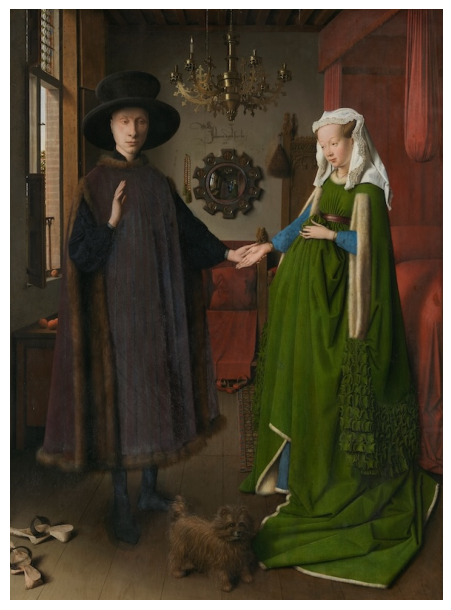

We also need to create a coordinate grid that represents the spatial coordinates of each pixel in the image. This grid will be the input to our neural network, and the target will be the RGB values of the corresponding pixels in the image. We’ll use the coordinate grid to train the model to predict the RGB values based on spatial location.

This grid looks as the following, notice that the image is inverted in the y-axis compared to the usual image representation. This is because the origin \((0,0)\) is at the top-left corner in the image, while in the Cartesian coordinate system it is at the bottom-left corner.

def create_coordinate_grid(H, W, device):
    x = np.linspace(0, 1, W)
    y = np.linspace(0, 1, H)
    xx, yy = np.meshgrid(x, y)
    coords = np.stack([xx, yy], axis=-1).reshape(-1, 2)
    return torch.FloatTensor(coords).to(device)


def create_target_tensor(img, device):
    return torch.FloatTensor(img.reshape(-1, 3)).to(device)


# Prepare coordinate grid and target tensor
coords = create_coordinate_grid(H, W, device)
target = create_target_tensor(img, device)

# Plot coordinate grid and target tensor
plt.figure(figsize=(8, 8))
plt.scatter(coords.cpu()[:, 0], coords.cpu()[:, 1], s=1, c=target.cpu())
plt.show()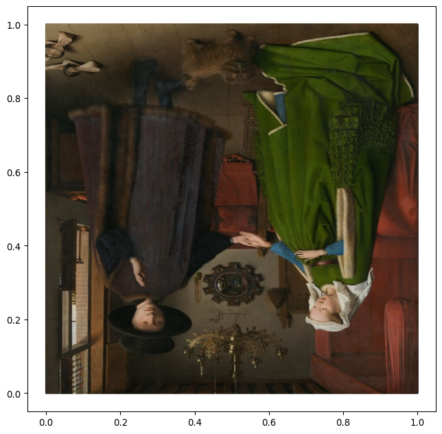

We also need to create directories to store the display and animation frames, this way we don’t have to store all the frames in memory. We’ll use these to save the model’s predictions at different epochs during training, which we will later use to create an animation of the training process.

import os

display_dir = "display_frames"
anim_dir = "animation_frames"
os.makedirs(display_dir, exist_ok=True)
os.makedirs(anim_dir, exist_ok=True)

The model

As mentioned before, we will use a Multi-Layer Perceptron (MLP) model. It features an input layer that accepts \((x,y)\) coordinates, three hidden layers with :link ReLU activation functions, and an output layer that produces the predicted RGB values. While an MLP is a basic neural network that may not capture complex spatial patterns as well as more advanced architectures, this very limitation helps visually highlight the optimizer’s struggle to learn the image, and how Adam adapts as it traverses the loss landscape.

from torch import nn


class MLP(nn.Module):
    def __init__(
        self, in_features=2, hidden_features=512, hidden_layers=3, out_features=3
    ):
        super(MLP, self).__init__()
        layers = [nn.Linear(in_features, hidden_features), nn.ReLU()]
        for _ in range(hidden_layers):
            layers.append(nn.Linear(hidden_features, hidden_features))
            layers.append(nn.ReLU())
        layers.append(nn.Linear(hidden_features, out_features))
        self.net = nn.Sequential(*layers)

    def forward(self, x):
        return self.net(x)

Note the model doesn’t have enough parameters to fully memorize the image and will struggle to capture the details of the painting pixel by pixel. This limitation will be evident in the animation, where the model’s predictions will be a blurry approximation of the original image. You can think of it as the model having to compress information into a lower-dimensional space and then reconstruct it, losing detail in the process. To produce an image that closely resembles the original, we would need a more complex architecture, a different approach, or lots of epochs to capture enough detail.

model_mlp = MLP(
    in_features=2,
    hidden_features=hidden_features,
    hidden_layers=hidden_layers,
    out_features=3,
).to(device)

print(model_mlp)
print(
    "Number of parameters:",
    sum(p.numel() for p in model_mlp.parameters() if p.requires_grad),
)

MLP(
  (net): Sequential(
    (0): Linear(in_features=2, out_features=512, bias=True)
    (1): ReLU()
    (2): Linear(in_features=512, out_features=512, bias=True)
    (3): ReLU()
    (4): Linear(in_features=512, out_features=512, bias=True)
    (5): ReLU()
    (6): Linear(in_features=512, out_features=512, bias=True)
    (7): ReLU()
    (8): Linear(in_features=512, out_features=512, bias=True)
    (9): ReLU()
    (10): Linear(in_features=512, out_features=3, bias=True)
  )
)
Number of parameters: 1053699

Finally we define the Adam optimiser and the Mean Squared Error (MSE) loss function. Remember the optimiser is responsible for updating the model’s parameters towards minimizing the loss function, while the MSE loss measures the difference between the model’s predictions and the target values (the original pixels), which we aim to minimize during training.

import torch.optim as optim

optimizer = optim.Adam(model_mlp.parameters(), lr=learning_rate)
criterion = nn.MSELoss()

With this out of the way, let us train the model and save the display and animation frames. We’ll also implement early stopping based on the patience hyper-parameter, which stops training if the loss does not improve for a certain number of epochs. If you decide to try this yourself, keep in mind that depending on your hardware, training may take a while (hours) due to the necessary large number of epochs and the complexity of the model.

from tqdm.notebook import tqdm


def save_frame(frame, folder, prefix, epoch):
    """Save a frame (as an image) to the given folder."""
    frame_path = os.path.join(folder, f"{prefix}_{epoch:04d}.png")
    # If frame is grayscale, use cmap; otherwise, display as color
    if frame.ndim == 2 or frame.shape[-1] == 1:
        plt.imsave(frame_path, frame.astype(np.float32), cmap="gray")
    else:
        plt.imsave(frame_path, frame.astype(np.float32))


def train_model(
    model,
    coords,
    target,
    H,
    W,
    num_epochs,
    display_interval,
    animation_interval,
    patience,
    optimizer,
    criterion,
    display_dir,
    anim_dir,
    create_animation,
):
    best_loss = float("inf")
    patience_counter = 0
    display_epochs = []
    display_losses = []

    for epoch in tqdm(range(num_epochs), desc="Training"):
        optimizer.zero_grad()
        pred = model(coords)
        loss = criterion(pred, target)
        loss.backward()
        optimizer.step()

        if loss.item() < best_loss:
            best_loss = loss.item()
            patience_counter = 0
        else:
            patience_counter += 1

        if patience_counter >= patience:
            print(f"Early stopping at epoch {epoch}, best loss: {best_loss:.6f}")
            break

        with torch.no_grad():
            # Reshape prediction to (H, W, 3) for a color image
            pred_img = pred.detach().cpu().numpy().astype(np.float16).reshape(H, W, 3)
            frame = np.clip(pred_img, 0, 1)

            if create_animation and epoch % animation_interval == 0:
                save_frame(frame, anim_dir, "frame", epoch)

            if epoch % display_interval == 0:
                save_frame(frame, display_dir, "display", epoch)
                display_epochs.append(epoch)
                display_losses.append(loss.item())

        del pred
    return best_loss, display_epochs, display_losses


best_loss_mlp, display_epochs_mlp, display_losses_mlp = train_model(
    model_mlp,
    coords,
    target,
    H,
    W,
    num_epochs,
    display_interval,
    animation_interval,
    patience,
    optimizer,
    criterion,
    display_dir,
    anim_dir,
    create_animation,
)

With the training complete, we can display the saved frames to get a sense of how the model’s predictions evolved over time. They show the model’s output at different epochs, with the epoch number and loss value displayed with each image. This visualisation helps us understand how the model learns to approximate the original image pixel by pixel.

import glob
import math
import re


def extract_number(f):
    s = os.path.basename(f)
    match = re.search(r"(\d+)", s)
    return int(match.group(1)) if match else -1


def grid_display(display_dir, display_epochs, display_losses, num_cols=5):
    # Use the custom key for natural sorting of filenames
    display_files = sorted(
        glob.glob(os.path.join(display_dir, "*.png")), key=extract_number
    )
    num_images = len(display_files)
    num_rows = math.ceil(num_images / num_cols)

    fig, axes = plt.subplots(num_rows, num_cols, figsize=(num_cols * 3, num_rows * 3))
    axes = axes.flatten() if num_images > 1 else [axes]
    for i, ax in enumerate(axes):
        if i < num_images:
            img_disp = plt.imread(display_files[i])
            ax.imshow(
                img_disp if img_disp.ndim == 3 else img_disp,
                cmap=None if img_disp.ndim == 3 else "gray",
            )
            ax.set_title(f"Epoch {display_epochs[i]}\nLoss: {display_losses[i]:.6f}")
            ax.axis("off")
        else:
            ax.axis("off")
    plt.tight_layout()
    plt.show()


grid_display(display_dir, display_epochs_mlp, display_losses_mlp)

def cleanup_frames(directory):
    files = glob.glob(os.path.join(directory, "*.png"))
    for file in files:
        os.remove(file)


cleanup_frames(display_dir)

To get an even better intuition, let us create an animation which shows predictions at different epochs. This animation will give us a dynamic view of the training process, illustrating how the model’s output evolves over time. We’ll use the imageio library to create an MP4 video from the saved frames.

from PIL import Image, ImageDraw, ImageFont
import imageio.v2 as imageio
import glob
import os
import numpy as np


def create_mp4_from_frames(anim_dir, mp4_filename, fps=10):
    # Use the custom sort key to ensure natural sorting of filenames
    anim_files = sorted(glob.glob(os.path.join(anim_dir, "*.png")), key=extract_number)
    frames = []
    font_size = 32

    try:
        font = ImageFont.truetype(r"OpenSans-Bold.ttf", font_size)
    except IOError:
        font = ImageFont.load_default()

    for file in anim_files:
        base = os.path.basename(file)
        try:
            parts = base.split("_")
            iteration = parts[-1].split(".")[0]
        except Exception:
            iteration = "N/A"

        frame_array = imageio.imread(file)
        image = Image.fromarray(frame_array)
        # Ensure image is in RGB mode for drawing colored text
        if image.mode != "RGB":
            image = image.convert("RGB")

        draw = ImageDraw.Draw(image)
        text = str(iteration)
        textwidth = draw.textlength(text, font)
        textheight = font_size

        width, height = image.size
        x = width - textwidth - 10
        y = height - textheight - 10

        # For RGB images, white is (255, 255, 255)
        draw.text((x, y), text, font=font, fill=(255, 255, 255))
        frames.append(np.array(image))

    # Write frames to an MP4 video file with the ffmpeg writer
    writer = imageio.get_writer(mp4_filename, fps=fps, codec="libx264", format="ffmpeg")
    for frame in frames:
        writer.append_data(frame)
    writer.close()

if create_animation:
    create_mp4_from_frames(anim_dir, "The_Arnolfini_portrait_RGB_MLP.mp4", fps=24)
    cleanup_frames(anim_dir)

We can clearly see the model slowly learn the details of the painting over time, starting from a verry blurry approximation and gradually refining its predictions. The role of the optimiser, is to guide the model towards “guessing” the details of the painting, such as textures, colours, and shapes. The “wiggles” in the animation represent the model’s attempt to find the optimal parameters that minimize the loss function, which in turn helps it produce more accurate predictions, just like when a person tries to find the optimal path around a complex maze by trial and error.

The SIREN model

MLPs, when used with standard activation functions like ReLU, tend to create piecewise linear approximations of the target function. This works well for many problems, but it can lead to over-smoothing when modeling complex spatial patterns, especially in images. Essentially, an MLP struggles to capture high-frequency details or subtle variations in an image because its architecture is inherently limited by its smooth, global parameterization.

On the other hand, a SIREN model, short for Sinusoidal Representation Networks, employs periodic activation functions (typically sine functions) instead of ReLU. The sinusoidal activations allow the network to naturally capture high-frequency details, as they can represent oscillatory patterns much more effectively. This means that it will be better suited for representing complex, detailed signals with fine variations, making it a strong candidate for tasks such as image reconstruction or any problem where precise spatial detail is critical. It will also help the optimizer converge much faster and more accurately to the target image.

import numpy as np
import matplotlib.pyplot as plt

x = np.linspace(-2 * np.pi, 2 * np.pi, 1000)


def relu(x):
    return np.maximum(0, x)


omega0 = 5.0  # frequency scaling factor


def siren(x):
    return np.sin(omega0 * x)


fig, (ax1, ax2) = plt.subplots(1, 2, figsize=(8, 4))

ax1.plot(x, relu(x), label="MLP (ReLU)", color="blue")
ax1.set_title("ReLU Activation")
ax1.set_xlabel("x")
ax1.set_ylabel("f(x)")
ax1.axhline(0, color="black", linewidth=0.5)
ax1.axvline(0, color="black", linewidth=0.5)
ax1.grid(True)
ax1.legend()

ax2.plot(x, siren(x), label="SIREN (sin activation)", color="red")
ax2.set_title("Sine Activation")
ax2.set_xlabel("x")
ax2.set_ylabel("f(x)")
ax2.axhline(0, color="black", linewidth=0.5)
ax2.axvline(0, color="black", linewidth=0.5)
ax2.grid(True)
ax2.legend()

plt.tight_layout()
plt.show()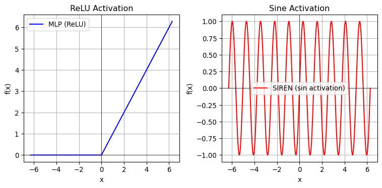

Here’s how SIREN is defined in PyTorch. The key difference is the use of the SineLayer class, which replaces the standard linear layers in the MLP. The SineLayer applies a sine function to the output of a linear layer, with a frequency controlled by the omega_0 parameter. The SIREN class then stacks multiple SineLayer instances to create a deep network with sinusoidal activations. The choice of omega_0 determines the frequency of the sine functions and can be tuned to capture different spatial frequencies in the data.

class SineLayer(nn.Module):
    def __init__(
        self, in_features, out_features, bias=True, is_first=False, omega_0=30
    ):
        super().__init__()
        self.in_features = in_features
        self.is_first = is_first
        self.omega_0 = omega_0
        self.linear = nn.Linear(in_features, out_features, bias=bias)
        self.init_weights()

    def init_weights(self):
        with torch.no_grad():
            if self.is_first:
                self.linear.weight.uniform_(-1 / self.in_features, 1 / self.in_features)
            else:
                self.linear.weight.uniform_(
                    -math.sqrt(6 / self.in_features) / self.omega_0,
                    math.sqrt(6 / self.in_features) / self.omega_0,
                )

    def forward(self, input):
        return torch.sin(self.omega_0 * self.linear(input))


class SIREN(nn.Module):
    def __init__(
        self, in_features, hidden_features, hidden_layers, out_features, omega_0=30
    ):
        super().__init__()
        layers = [
            SineLayer(in_features, hidden_features, is_first=True, omega_0=omega_0)
        ]
        for _ in range(hidden_layers):
            layers.append(
                SineLayer(
                    hidden_features, hidden_features, is_first=False, omega_0=omega_0
                )
            )
        final_linear = nn.Linear(hidden_features, out_features)
        with torch.no_grad():
            final_linear.weight.uniform_(
                -math.sqrt(6 / hidden_features) / omega_0,
                math.sqrt(6 / hidden_features) / omega_0,
            )
        layers.append(final_linear)
        self.net = nn.Sequential(*layers)

    def forward(self, x):
        return self.net(x)

Together with the model, we also recreate the optimizer with the same hyper-parameters as before.

model_siren = SIREN(
    in_features=2,
    hidden_features=hidden_features,
    hidden_layers=hidden_layers,
    out_features=3,
).to(device)

optimizer = optim.Adam(model_siren.parameters(), lr=learning_rate)
criterion = nn.MSELoss()

Finally, we run training and save the display and animation frames. This time we should see convergence being achieved faster, and more detailed predictions compared to the MLP, thanks to SIREN’s ability to capture high-frequency spatial patterns more effectively.

animation_interval = 5  # SIREN converges much faster
display_interval = 200
patience = 200

best_loss_siren, display_epochs_siren, display_losses_siren = train_model(
    model_siren,
    coords,
    target,
    H,
    W,
    num_epochs,
    display_interval,
    animation_interval,
    patience,
    optimizer,
    criterion,
    display_dir,
    anim_dir,
    create_animation,
)

Early stopping at epoch 3084, best loss: 0.000131

As before let us see the display frames to get an idea of how the model’s predictions evolved over time before converging.

grid_display(display_dir, display_epochs_siren, display_losses_siren)
cleanup_frames(display_dir)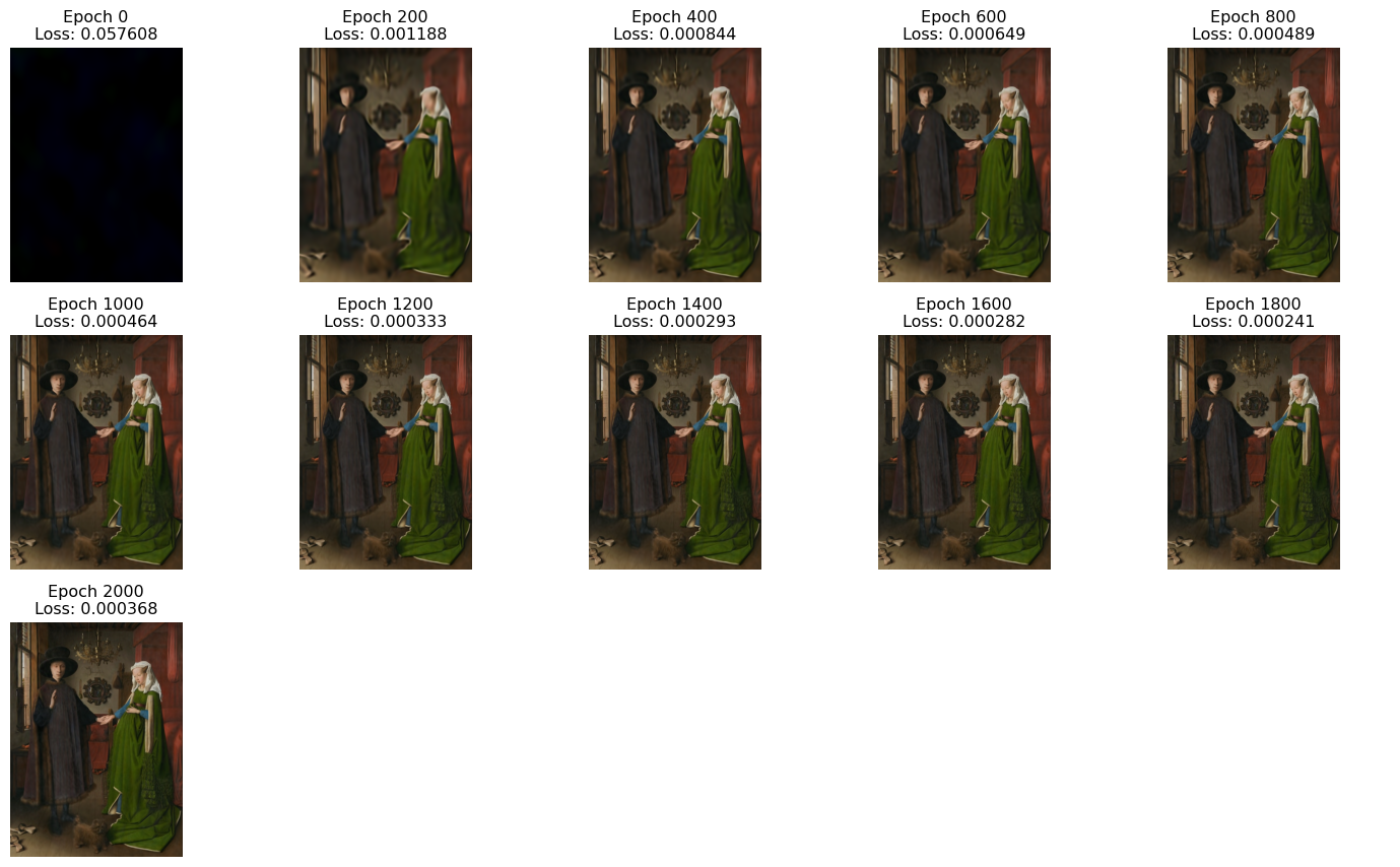

And finally stich the animation frames together to create a video that shows the training process of the SIREN model.

if create_animation:
    create_mp4_from_frames(anim_dir, "The_Arnolfini_portrait_RGB_SIREN.mp4", fps=12)
    cleanup_frames(anim_dir)

Notice how this time SIREN captures fine details much faster and accurately than the MLP. It has almost memorized the training data, showing the effectiveness of SIREN in high-frequency function representation. The Adam optimizer, in this case, has an easier time navigating the loss landscape, converging to the target image much faster and with more precision.

Final remarks

Hopefully this experiment has given you a better understanding of the role of optimisation in machine learning, it is a crucial aspect that affects how well models perform and converge during training, and despite the somewhat complex nature of the algorithms employed, it is possible for anyone to get a rough intuition of how they work.