random forests and embeddings for sentiment analysis
Experiments
Machine Learning
NLP
Published
June 19, 2024
Natural language processing (NLP) is often associated with deep learning and neural networks. However, there are efficient methods for text classification that do not rely on neural networks. In this exploration, we will demonstrate a sentiment analysis classification problem using text embeddings combined with traditional machine learning algorithms.
The task at hand is sentiment analysis: classifying tweets as positive, negative, neutral, or irrelevant. Sentiment analysis determines the emotional tone of text. Although neural networks, particularly models like BERT, are popular for this task, traditional machine learning algorithms can also be effective when used with modern text embeddings.
We will use a Twitter dataset containing labeled tweets to classify their sentiment. Our approach involves using the BERT tokenizer and embeddings (we previously looked at the basics of embeddings) for text preprocessing, followed by traditional machine learning algorithms for classification.
Using traditional machine learning algorithms offers several advantages. They are generally faster and require less computational power compared to deep learning models, making them suitable for resource-limited scenarios. Additionally, traditional algorithms are often easier to interpret, providing more transparency in decision-making processes. Moreover, traditional algorithms can achieve competitive performance when combined with powerful text embeddings like those from BERT.
Loading and understanding the data
Let’s start by loading the dataset and understanding its structure. The dataset contains tweets labeled as positive, negative, neutral, or irrelevant. We will load the data and examine a few samples to understand the text and labels.
Show the code
# Download the dataset!kaggle datasets download -d jp797498e/twitter-entity-sentiment-analysis -p .data/--unzip
Warning: Looks like you're using an outdated API Version, please consider updating (server 1.7.4.2 / client 1.6.17)
Dataset URL: https://www.kaggle.com/datasets/jp797498e/twitter-entity-sentiment-analysis
License(s): CC0-1.0
Downloading twitter-entity-sentiment-analysis.zip to .data
  0%|                                               | 0.00/1.99M [00:00<?, ?B/s] 50%|███████████████████                   | 1.00M/1.99M [00:00<00:00, 4.72MB/s]100%|██████████████████████████████████████| 1.99M/1.99M [00:00<00:00, 5.88MB/s]
100%|██████████████████████████████████████| 1.99M/1.99M [00:00<00:00, 5.67MB/s]
Note how the Irrelevant category has the least number of samples, which might pose a challenge for training a classifier. Let us also check the category distribution for the validation set.
Before continuing, we will also drop any rows with missing values in the text column.
Show the code
# Validate that 'text' is not null or emptysentiment = sentiment.dropna(subset=["text"])sentiment_validation = sentiment_validation.dropna(subset=["text"])
Calculating embeddings using BERT
We will be using the BERT model for generating embeddings for the text data. BERT (Bidirectional Encoder Representations from Transformers) is a powerful pre-trained language model that can be fine-tuned for various NLP tasks. In this case, we will use BERT to generate embeddings for the tweets in our dataset.
We have explored BERT embeddings in a previous experiment. As reference, in that experiment, a fine tuned BERT model achieved an accuracy of 0.87.
Show the code
import torchfrom transformers import BertTokenizer, BertModelimport pytorch_lightning as plimport pandas as pd# Define a LightningModule that wraps the BERT model and tokenizerclass BERTEmbeddingModule(pl.LightningModule):def__init__(self):super().__init__()self.tokenizer = BertTokenizer.from_pretrained("bert-base-uncased")self.bert_model = BertModel.from_pretrained("bert-base-uncased")def forward(self, texts):# Tokenize the input texts inputs =self.tokenizer( texts, return_tensors="pt", truncation=True, padding=True, max_length=512 )# Ensure inputs are on the same device as the model device =next(self.parameters()).device inputs = {k: v.to(device) for k, v in inputs.items()} outputs =self.bert_model(**inputs)# Average the last hidden state over the sequence length dimension embeddings = outputs.last_hidden_state.mean(dim=1)return embeddings# Determine the device: CUDA, MPS, or CPUif torch.cuda.is_available(): device = torch.device("cuda")elif torch.backends.mps.is_available(): device = torch.device("mps")else: device = torch.device("cpu")print(f"Using device: {device}")# Initialize the model, move it to the correct device, and set it to evaluation modebert_model = BERTEmbeddingModule()bert_model.to(device)bert_model.eval()# Convert text columns to listssentiment_texts = sentiment["text"].tolist()sentiment_validation_texts = sentiment_validation["text"].tolist()batch_size =64# Compute embeddings in batches for the sentiment DataFramesentiment_embeddings = []with torch.no_grad():for i inrange(0, len(sentiment_texts), batch_size): batch_texts = sentiment_texts[i : i + batch_size] batch_embeddings = bert_model(batch_texts) sentiment_embeddings.extend(batch_embeddings.cpu().numpy())if (i // batch_size) %20==0:print(f"Processed {i} sentences", end="\r")# Add the embeddings to the sentiment DataFramesentiment = sentiment.assign(embedding=sentiment_embeddings)# Compute embeddings in batches for the sentiment_validation DataFramesentiment_validation_embeddings = []with torch.no_grad():for i inrange(0, len(sentiment_validation_texts), batch_size): batch_texts = sentiment_validation_texts[i : i + batch_size] batch_embeddings = bert_model(batch_texts) sentiment_validation_embeddings.extend(batch_embeddings.cpu().numpy())if (i // batch_size) %20==0:print(f"Processed {i} validation sentences", end="\r")# Add the embeddings to the sentiment_validation DataFramesentiment_validation = sentiment_validation.assign( embedding=sentiment_validation_embeddings)
Let’s check what the embeddings look like for a sample tweet.
Show the code
# Show a few random samples of the sentiment DataFramesentiment.sample(3, random_state=42)
id
tag
sentiment
text
embedding
61734
4984
GrandTheftAuto(GTA)
Irrelevant
Do you think you can hurt me?
[0.08892428, 0.26482618, -0.067467935, -0.0081...
11260
13136
Xbox(Xseries)
Positive
About The time!!
[0.17830487, -0.098808326, 0.3218802, -0.05973...
55969
11207
TomClancysRainbowSix
Neutral
Calls from _ z1rv _ & @ Tweet98 got me this so...
[0.16375753, -0.028547525, 0.36362433, -0.0574...
Notice the computed embedding vector for the tweet. This vector captures the semantic information of the text, which can be used as input for traditional machine learning algorithms. Let us look at the embedding in more detail.
Show the code
# Show the first 20 embedding values for row 0 of the sentiment DataFrame, and its shapeprint(sentiment.loc[0, "embedding"][:20])print(sentiment.loc[0, "embedding"].shape)
The embedding vector has 768 dimensions, encoding the semantic information of the text data. Different models may have different embedding dimensions, but BERT embeddings are typically 768 or 1024 dimensions.
Let us also drop the tag and id columns from the training and validation sets, as they are not needed for classification.
Show the code
# Drop the 'tag' and 'id' columnssentiment = sentiment.drop(columns=["tag", "id"])sentiment_validation = sentiment_validation.drop(columns=["tag", "id"])
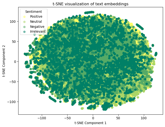
And finally before we continue, let us evaluate the degree of separation between the classes in the embedding space. We will use t-SNE to visualize the embeddings in 2D space.
Show the code
# Plot a t-SNE visualization of the embeddingsfrom sklearn.manifold import TSNEimport matplotlib.pyplot as pltimport numpy as np# Copy the sentiment DataFrame to avoid modifying the originalsentiment_tsne = sentiment.copy()# Convert sentiment labels to numerical valuessentiment_tsne["sentiment_num"] = sentiment["sentiment"].astype("category").cat.codes# Compute a t-SNE embedding of the embeddingstsne = TSNE(n_components=2)tsne_results = tsne.fit_transform(np.stack(sentiment_tsne["embedding"]))# Plot the t-SNE visualizationplt.figure(figsize=(8, 6))# Map the numerical values back to the original sentiment labelsunique_sentiments = sentiment_tsne["sentiment"].unique()colors = plt.cm.summer_r(np.linspace(0, 1, len(unique_sentiments)))# Create a scatter plot with a legendfor i, sentiment_label inenumerate(unique_sentiments): indices = sentiment_tsne["sentiment"] == sentiment_label plt.scatter( tsne_results[indices, 0], tsne_results[indices, 1], label=sentiment_label, c=[colors[i]], alpha=0.5, )plt.xlabel("t-SNE Component 1")plt.ylabel("t-SNE Component 2")plt.title("t-SNE visualization of text embeddings")plt.legend(title="Sentiment")plt.show()
It’s hard to discern much separation between the classes in the 2D t-SNE plot. This suggests that the classes are not easily separable in the embedding space, which might pose a challenge for classification.
Evaluating traditional machine learning algorithms
In this experiment, we will evaluate the performance of both Random Forest and XGBoost classifiers on the dataset. We will train these classifiers on the BERT embeddings and evaluate their performance on the validation set.
Both Random Forest and XGBoost are powerful ensemble learning algorithms that can handle high-dimensional data but may be prone to overfitting. We will tune their hyperparameters using grid search to optimize performance.
About Cross validation
Cross-validation is a technique used in machine learning to assess how a model will generalize to an independent dataset. It involves partitioning the original dataset into a set of training and validation subsets. The most common form of cross-validation is k-fold cross-validation, where the dataset is randomly divided into \(\mathbf{k}\) equally sized folds.
The model is trained on \(\mathbf{k-1}\) folds and tested on the remaining fold. This process is repeated \(\mathbf{k}\) times, with each fold serving as the validation set once. The performance metric (such as accuracy, precision, recall, or mean squared error) is averaged over the k iterations to provide a more robust estimate of the model’s performance.
This method helps in detecting overfitting and ensures that the model’s evaluation is not overly dependent on a particular subset of the data. By using cross-validation, one can make better decisions about model selection and hyperparameter tuning, leading to more reliable and generalizable models.
Show the code
import numpy as npfrom sklearn.ensemble import RandomForestClassifierfrom xgboost import XGBClassifierfrom sklearn.metrics import classification_report, accuracy_score, make_scorer, f1_scorefrom sklearn.model_selection import train_test_split, GridSearchCVfrom sklearn.preprocessing import LabelEncoderfrom sklearn.base import BaseEstimator, ClassifierMixin# Define a wrapper class for XGBoost, so we can keep categories as stringsclass XGBClassifierWrapper(BaseEstimator, ClassifierMixin):def__init__(self, **params):self.params = paramsself.model = XGBClassifier(**params)self.label_encoder = LabelEncoder()def fit(self, X, y): y_encoded =self.label_encoder.fit_transform(y)self.classes_ =self.label_encoder.classes_self.model.set_params(**self.params)self.model.fit(X, y_encoded)returnselfdef predict(self, X): y_pred =self.model.predict(X)returnself.label_encoder.inverse_transform(y_pred)def predict_proba(self, X):returnself.model.predict_proba(X)def get_params(self, deep=True):returnself.paramsdef set_params(self, **params):self.params.update(params)self.model.set_params(**self.params)returnself# Extract features (embeddings) and labelsX = np.vstack(sentiment["embedding"].values)y = sentiment["sentiment"].values# Split the dataset into training and test setsX_train, X_test, y_train, y_test = train_test_split( X, y, test_size=0.2, random_state=42)# Define the classifiers and their respective parameter gridsclassifiers = {"RandomForest": RandomForestClassifier(random_state=42, n_jobs=-1),"XGBoost": XGBClassifierWrapper(),}param_grids = {"RandomForest": {"n_estimators": [200, 300],"max_depth": [10, 20],"min_samples_split": [2, 5],"min_samples_leaf": [1, 5], },"XGBoost": {"n_estimators": [200, 300],"max_depth": [3, 6],"reg_alpha": [0, 0.1], # L1 regularization term on weights"reg_lambda": [1, 2], # L2 regularization term on weights },}# Define a custom scoring function that balances precision, recall, and accuracyscoring = {"accuracy": "accuracy", "f1": make_scorer(f1_score, average="weighted")}# Perform grid search for each classifier, and store the best modelsbest_models = {}for name, clf in classifiers.items():# Perform grid search with cross-validation, using f1 score as the metric (balancing precision and recall) grid_search = GridSearchCV( clf, param_grids[name], cv=3, scoring=scoring, n_jobs=-1, verbose=1, refit="f1" ) grid_search.fit(X_train, y_train) best_models[name] = grid_search.best_estimator_print(f"{name} best parameters:", grid_search.best_params_)
Fitting 3 folds for each of 16 candidates, totalling 48 fits
RandomForest best parameters: {'max_depth': 20, 'min_samples_leaf': 1, 'min_samples_split': 2, 'n_estimators': 300}
Fitting 3 folds for each of 16 candidates, totalling 48 fits
We trained both Random Forest and XGBoost classifiers on the training set. We used the F1 score as the evaluation metric, as it provides a balance between precision and recall. The F1 score is particularly useful for imbalanced datasets, like the one we have, where the number of samples in each class is not equal. In particular, we used L1 and L2 regularization for XGBoost to prevent overfitting.
Now, we will evaluate the performance of the Random Forest and XGBoost classifiers on the validation set to choose the best performing model.
Show the code
# Validation setX_val = np.vstack(sentiment_validation["embedding"].values)y_val = sentiment_validation["sentiment"].valuesprint(X_val.shape)print(y_val.shape)# Evaluate the best models on the validation set and choose the best onebest_model =Nonebest_accuracy =0for name, model in best_models.items(): y_val_pred = model.predict(X_val) accuracy_val = accuracy_score(y_val, y_val_pred) report_val = classification_report(y_val, y_val_pred)print(f"Validation Accuracy for {name}: {accuracy_val}")print(f"Classification Report for {name}:\n{report_val}\n")if accuracy_val > best_accuracy: best_accuracy = accuracy_val best_model = model best_y_val_pred = y_val_predprint(f"Best Model: {best_model}")print(f"Best Validation Accuracy: {best_accuracy}")
The XGBoost classifier outperforms the Random Forest classifier on the validation set, achieving an F1 score of 0.81, significantly higher than the Random Forest’s F1 score of 0.74.
About the F1 score
The F1 score is a metric that combines precision and recall into a single value. It is calculated as the harmonic mean of precision and recall:
The F1 score ranges from 0 to 1, with 1 being the best possible score. It is particularly useful when dealing with imbalanced datasets, as it provides a balance between precision and recall. A high F1 score indicates that the classifier has both high precision and high recall, making it a good choice for evaluating models on imbalanced datasets.
The Irrelevant class has the lowest F1-score, which is expected given the class imbalance in the dataset. Removing the Irrelevant class from the dataset, or merging it with Neutral would improve the overall performance of the classifier by quite a few points.
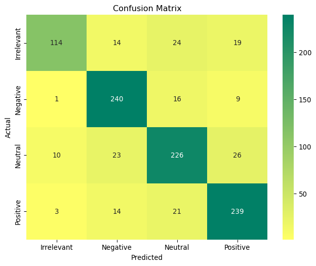
The confusion matrix for the XGBoost classifier on the validation set looks as follows:
Show the code
# Plot a confusion matrix with a summer_r colormapimport matplotlib.pyplot as pltimport seaborn as snsfrom sklearn.metrics import confusion_matrixcm = confusion_matrix(y_val, best_y_val_pred)plt.figure(figsize=(8, 6))sns.heatmap( cm, annot=True, fmt="d", cmap="summer_r", xticklabels=best_model.classes_, yticklabels=best_model.classes_,)plt.xlabel("Predicted")plt.ylabel("Actual")plt.title("Confusion Matrix")plt.show()
As expected, the Irrelevant class has the lowest precision and recall, while the Positive class has the highest precision and recall. The confusion matrix provides a detailed breakdown of the classifier’s performance on each class.
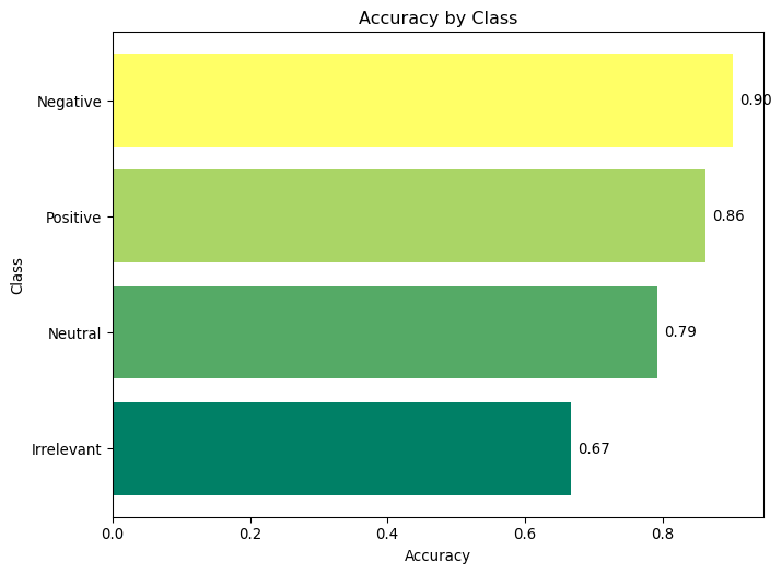
Let us also calculate the per-class accuracy for the XGBoost classifier on the validation set.
Show the code
# Plot accuracy for each classimport matplotlib.pyplot as pltfrom sklearn.metrics import accuracy_scoreimport numpy as np# Calculate accuracy for each classclass_accuracies = {}for i, class_name inenumerate(best_model.classes_): class_accuracies[class_name] = accuracy_score( y_val[y_val == class_name], best_y_val_pred[y_val == class_name] )# Sort classes by accuracyclass_accuracies =dict(sorted(class_accuracies.items(), key=lambda x: x[1], reverse=True))# Plot accuracy for each class using summer_r colormapplt.figure(figsize=(8, 6))colors = plt.cm.summer_r(np.linspace(0, 1, len(class_accuracies)))bars = plt.barh(list(class_accuracies.keys()), list(class_accuracies.values()), color=colors)# Add accuracy values to each color barfor bar in bars: width = bar.get_width() plt.text( width +0.01, bar.get_y() + bar.get_height() /2, f"{width:.2f}", va="center" )plt.xlabel("Accuracy")plt.ylabel("Class")plt.title("Accuracy by Class")plt.gca().invert_yaxis() # Invert y-axis to have the highest accuracy at the topplt.show()
And finally let us evaluate the performance of the XGBoost classifier on a set of entirely new, general sentences. These are sentences that the model has not seen before or which originate from the original dataset, and will help us understand how well the model generalizes to unseen data.
Show the code
import numpy as npfrom sklearn.metrics import accuracy_score# Test sentences with their corresponding true sentiments (Positive/Negative/Neutral/Irrelevant)test_sentences = [ ("This ice cream is delicious!", "Positive"), ("I hate this phone.", "Negative"), ("I love this car.", "Positive"), ("I don't like this book.", "Negative"), ("This sandwich couldn't be worse!", "Negative"), ("I'm in love with this song.", "Positive"), ("Why is this happening to me?", "Negative"), ("This is the worst day ever.", "Negative"), ("Ha! Ha! Ha! This is so funny", "Positive"), ("I'm so sad right now.", "Negative"), ("That phone really sucks.", "Negative"), ("What a fantastic performance!", "Positive"), ("This place is amazing!", "Positive"), ("I'm extremely disappointed in this service.", "Negative"), ("This is the best thing ever!", "Positive"), ("I can't stand this anymore.", "Negative"), ("This movie is a masterpiece.", "Positive"), ("I feel utterly miserable.", "Negative"), ("What a wonderful surprise!", "Positive"), ("This is a total disaster.", "Negative"), ("I'm thrilled with the results.", "Positive"), ("I detest this kind of behavior.", "Negative"), ("This experience was phenomenal.", "Positive"), ("I regret buying this product.", "Negative"), ("I'm ecstatic about the news!", "Positive"), ("This is utterly ridiculous.", "Negative"), ("I couldn't be happier with my decision.", "Positive"), ("This is an absolute failure.", "Negative"), ("I'm over the moon with joy!", "Positive"), ("This is the last straw.", "Negative"), ("I'm feeling great today!", "Positive"), ("This product is amazing!", "Positive"), ("I'm very unhappy with this.", "Negative"), ("What a terrible experience!", "Negative"), ("This is just perfect.", "Positive"), ("I love the way this looks.", "Positive"), ("I'm so frustrated right now.", "Negative"), ("This is absolutely fantastic!", "Positive"), ("I can't believe how bad this is.", "Negative"), ("I'm delighted with the outcome.", "Positive"), ("This is so disappointing.", "Negative"), ("What a lovely day!", "Positive"), ("I'm completely heartbroken.", "Negative"), ("This is pure bliss.", "Positive"), ("I despise this kind of thing.", "Negative"), ("I'm overjoyed with the results.", "Positive"), ("This is simply dreadful.", "Negative"), ("I'm very pleased with this.", "Positive"), ("This is a nightmare.", "Negative"), ("I'm so happy right now!", "Positive"), ("This is not acceptable.", "Negative"), ("I'm really enjoying this.", "Positive"), ("This is absolutely horrible.", "Negative"), ("I love spending time here.", "Positive"), ("This is the most frustrating thing ever.", "Negative"), ("I'm incredibly satisfied with this.", "Positive"), ("This is a complete mess.", "Negative"), ("What an extraordinary event!", "Positive"), ("This is beyond disappointing.", "Negative"), ("I'm elated with my progress.", "Positive"), ("This is such a waste of time.", "Negative"), ("I'm absolutely thrilled!", "Positive"), ("This situation is unbearable.", "Negative"), ("I can't express how happy I am.", "Positive"), ("This is a total failure.", "Negative"), ("I'm so grateful for this opportunity.", "Positive"), ("This is driving me crazy.", "Negative"), ("I'm in awe of this beauty.", "Positive"), ("This is utterly pointless.", "Negative"), ("I'm having the time of my life!", "Positive"), ("This is so infuriating.", "Negative"), ("I absolutely love this place.", "Positive"), ("This is the worst experience ever.", "Negative"), ("I'm overjoyed to be here.", "Positive"), ("This is a huge disappointment.", "Negative"), ("I'm very content with this.", "Positive"), ("This is the most annoying thing.", "Negative"), ("I'm extremely happy with the results.", "Positive"), ("This is totally unacceptable.", "Negative"), ("I'm so excited about this!", "Positive"), ("This is very upsetting.", "Negative"), ("The sky is blue.", "Neutral"), ("Water is wet.", "Neutral"), ("I have a meeting tomorrow.", "Irrelevant"), ("The cat is on the roof.", "Neutral"), ("I'm planning to go shopping.", "Irrelevant"), ("This text is written in English.", "Neutral"), ("It's raining outside.", "Neutral"), ("I need to buy groceries.", "Irrelevant"), ("My favorite color is blue.", "Neutral"), ("I watched a movie yesterday.", "Irrelevant"), ("Grass is green.", "Neutral"), ("The sun rises in the east.", "Neutral"), ("I need to finish my homework.", "Irrelevant"), ("Birds are chirping.", "Neutral"), ("I'm thinking about dinner.", "Irrelevant"), ("Trees provide oxygen.", "Neutral"), ("I'm planning a trip next week.", "Irrelevant"), ("The earth orbits the sun.", "Neutral"), ("I have to call my friend.", "Irrelevant"), ("The book is on the table.", "Neutral"), ("I need to wash the dishes.", "Irrelevant"),]def get_embedding(model, text): model.eval()with torch.no_grad():# Wrap the single text in a list since our forward method expects a list of texts embedding = model([text])return embedding.cpu().numpy().squeeze()# Separate the sentences and their true sentimentssentences, true_sentiments =zip(*test_sentences)# Generate embeddings for the test sentencestest_embeddings = np.array( [get_embedding(bert_model, sentence) for sentence in sentences])# Predict the sentiments using the trained modelpredictions = best_model.predict(test_embeddings)# Print the results and calculate accuracycorrect_predictions =0for sentence, true_sentiment, prediction inzip( sentences, true_sentiments, predictions): is_correct = prediction == true_sentimentif is_correct: correct_predictions +=1# Calculate and print the accuracyaccuracy = correct_predictions /len(sentences)print(f"Accuracy: {accuracy *100:.2f}%, for {correct_predictions}/{len(sentences)} correct predictions.")
Accuracy: 70.59%, for 72/102 correct predictions.
Final remarks
In this exploration, we demonstrated the effectiveness of traditional machine learning algorithms when combined with modern text embeddings for sentiment analysis. While deep learning models like BERT have set a high standard in NLP tasks, traditional algorithms such as Random Forest and XGBoost can still achieve competitive performance with significantly lower computational requirements.
Traditional machine learning algorithms are generally faster and require less computational power compared to deep learning models, making them suitable for scenarios where computational resources are limited. Additionally, traditional algorithms offer more transparency, allowing us to better understand how decisions are made. This is particularly valuable in applications where model interpretability is crucial.
When paired with powerful text embeddings like those generated by BERT, traditional machine learning algorithms can deliver strong performance. Our experiments showed that XGBoost, in particular, outperformed Random Forest in terms of accuracy and F1 score on the validation set. The challenge of class imbalance was evident in the lower performance of the Irrelevant class, and techniques such as re-sampling, cost-sensitive learning, or refining the model’s hyperparameters could further improve performance in future studies.
The methodology presented is practical and can be easily adapted to various text classification problems beyond sentiment analysis. This flexibility underscores the value of combining traditional machine learning algorithms with modern text embeddings.