how to log, compare, and deploy machine learning models consistently with mlflow
HowTo
Machine Learning
Model Management
Published
November 12, 2024
As you develop machine learning models, you will find that you need to manage many different versions and variations as you move towards the desired outcome. You may want to compare, roll back to previous versions, or deploy multiple versions of a model to A/B test which one is better. MLflow is one of many tools and frameworks that helps you manage this process. There are lots of alternatives in this space, including Kubeflow, DVC, and Metaflow.
Here we are looking at MLflow specifically because it is a lightweight, open-source platform that integrates with many popular machine learning libraries, including TensorFlow, PyTorch, and scikit-learn. It also has a simple API that makes it easy to log metrics, parameters, and artifacts (like models) from your machine learning code - helping you start tracking your experiments quickly with as little fuss as possible.
We will not cover all of MLflow’s features, only the basic functionality that you need to get started. If you want to learn more about MLflow, you can check out the official documentation.
Installation
Just install the mlflow package either with pip or conda, and you are good to go. It comes with a built-in tracking server that can run locally, or you can use a cloud-based tracking server, including ones provided as part of Azure ML and AWS SageMaker.
Unless otherwise specified, mlflow will log your experiments to a local directory called mlruns. To start the tracking server, run the following command:
mlflow server
A server will start on http://127.0.0.1:5000. You can access the UI by navigating to that URL in your browser.
Logging experiments
In a machine learning workflow, keeping a detailed log of parameters, metrics, and artifacts (such as trained models) for each experiment is crucial for ensuring reproducibility, performance monitoring, and informed decision-making. Without proper logging, comparing models, identifying improvements, and debugging issues become significantly more difficult.
MLflow simplifies this process with a user-friendly API that allows you to systematically track every aspect of your experiments. By logging parameters, such as learning rates and model architectures, along with evaluation metrics and model artifacts, it helps create a structured and searchable record of your work. This ensures that you can not only reproduce past results but also analyze trends over time, making it easier to identify what works best.
Beyond individual experimentation, proper logging is essential for collaboration. Whether you’re working alone or in a team, having a well-documented history of model runs makes it easier to share insights, compare different approaches, and troubleshoot unexpected results. If you work in a regulated industry, logging is also a key part of ensuring compliance with whatever regulations apply to your work.
A simple example
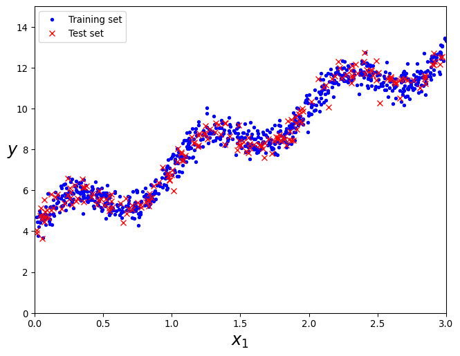
Let’s exemplify how to use MLflow with a simple use case. We will produce a 2D dataset, and train a variety of models on it. We will log the models, along with their hyperparameters and performance metrics to MLflow so we can reproduce and compare them later.
Show the code
import numpy as npimport matplotlib.pyplot as plt# Create a simple datasetnp.random.seed(42)X =3* np.random.rand(1000, 1)# Produce a sinusoidal curve with some noisey =4+3* X + np.sin(2* np.pi * X) +0.4* np.random.randn(1000, 1)
With the necessary dataset out of the way, we can now move on to creating an MLflow experiment. An experiment is a set of runs that are typically related to a specific goal. For example, you might create an experiment to compare different models on a specific dataset or to optimize a model for a specific metric. Each run within an experiment logs metrics, parameters, and artifacts, which can be compared and analyzed later.
Below, when we run autolog(), we are priming MLflow to automatically log all the parameters, metrics, model signatures, models and datasets from our runs. This is a convenient way to ensure that all relevant information is captured without having to manually log each item. It is the easiest way to get started, but you can also log items manually if you prefer.
Show the code
from mlflow import set_experimentfrom mlflow.sklearn import autolog# Name the experimentset_experiment("sinusoidal_regression")autolog( log_input_examples=True, log_model_signatures=True, log_models=True, log_datasets=True,)
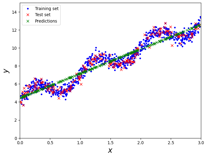
With the initial setup complete, we can now train a simple linear regression model on the dataset. You start a run typically with an expression of the form with mlflow.start_run():. This creates a new run within the active experiment which you’ve setup before, logging all the relevant information for that run. We can then train the model, and MLflow will ensure all relevant information is captured.
Anything that runs within the with block will be logged automagically. MLflow supports a wide range of machine learning frameworks - including TensorFlow, PyTorch (via Lightning), and scikit-learn. This includes libraries such as XGBoost or LightGBM as well.
Note
Always ensure you end your run with mlflow.end_run(). This will ensure that all the relevant information is logged to MLflow.
Show the code
# Create a simple linear regression modelfrom sklearn.linear_model import LinearRegressionfrom mlflow import start_run, set_tag, end_run, log_artifact, log_figurewith start_run(run_name="linear_regression") as run: set_tag("type", "investigation") lin_reg = LinearRegression() lin_reg.fit(train_set[["X"]], train_set["y"])# Make a prediction with some random data points y_pred = lin_reg.predict(test_set[["X"]])# Plot the prediction, include markers for the predicted data points fig, ax = plt.subplots(figsize=(8, 6)) ax.plot(train_set["X"], train_set["y"], "b.") ax.plot(test_set["X"], test_set["y"], "rx") ax.plot(test_set["X"], y_pred, "gx") ax.set_xlabel("$x$", fontsize=18) ax.set_ylabel("$y$", fontsize=18) ax.axis([0, 3, 0, 15]) ax.legend(["Training set", "Test set", "Predictions"])# Log the figure directly to MLflow log_figure(fig, "training_test_plot.png") plt.show() plt.close(fig) end_run()
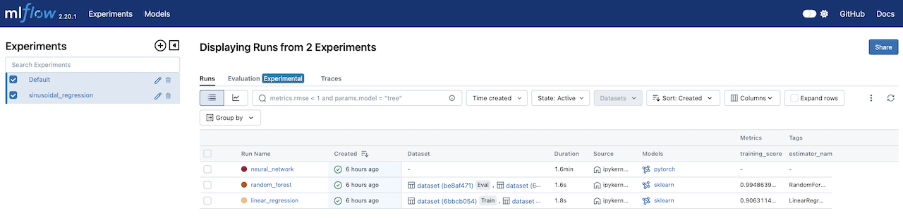
With the run finished, you can view the results in the MLflow UI. You will find the parameters, metrics, and artifacts logged for the run, compare runs, search them, and view their history within each experiment.
MLflow UI
With the data recorded, we can use the client API to query the data logged, for example, we can retrieve logged metrics for the run we just completed.
Show the code
from mlflow import MlflowClient# Use the MlflowClient to fetch the run detailsclient = MlflowClient()run_data = client.get_run(run.info.run_id).data# Extract and display the metricsmetrics = run_data.metricsprint("Logged Evaluation Metrics:")for metric, value in metrics.items():print(f"{metric}: {value}")
We can continue to log more runs to the same experiment, and compare the results in the MLflow UI. For example, let’s create another run, this time with a Random Forest regressor model. Notice that the flow of the code is the same as before, we start a new run, train the model and end the run.
We have so far relied on MLflow’s autologging feature to capture all the relevant information for our runs. However, you can also log items manually if you prefer. This gives more control over what is logged, and allows you to log custom metrics, parameters, and artifacts.
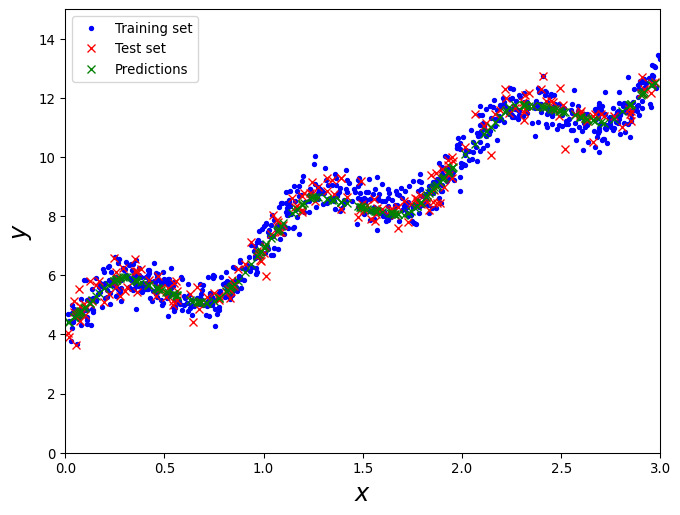
Let’s add another run to the experiment, this time logging the model manually. We will use a simple neural network model with PyTorch, but this time all logging will be setup explicitly instead of relying on autologging.
We start by setting up the network and model.
Show the code
# Predict with a PyTorch neural networkfrom torch import nn, device, backends, from_numpy, optimimport torchimport torch.nn.functional as Fdevice = torch.device("mps"if torch.mps.is_available() else"cpu")device = torch.device("cuda"if torch.cuda.is_available() else device)print(f"Using device: {device}")class NeuralNetwork(nn.Module):def__init__(self):super().__init__()self.flatten = nn.Flatten()self.linear_relu_stack = nn.Sequential( nn.Linear(1, 512), nn.ReLU(), nn.Linear(512, 512), nn.ReLU(), nn.Linear(512, 1), )def forward(self, x): x =self.flatten(x) logits =self.linear_relu_stack(x)return logits# Convert the data to PyTorch tensorsX_train = from_numpy(train_set["X"].values).float().view(-1, 1).to(device)y_train = from_numpy(train_set["y"].values).float().view(-1, 1).to(device)X_test = from_numpy(test_set["X"].values).float().view(-1, 1).to(device)y_test = from_numpy(test_set["y"].values).float().view(-1, 1).to(device)params = {"epochs": 500,"learning_rate": 1e-3,"batch_size": 8,"weight_decay": 1e-4,}# Define the neural network, loss function, and optimizermodel = NeuralNetwork().to(device)loss_fn = nn.MSELoss()optimizer = optim.Adam( model.parameters(), lr=params["learning_rate"], weight_decay=params["weight_decay"])params.update( {"loss_function": loss_fn.__class__.__name__,"optimizer": optimizer.__class__.__name__, })
Using device: cuda
We then start a new run, just like before, except that now we are logging everything manually - for example, using mlflow.log_params to log the hyperparameters, and mlflow.log_metrics for performance metrics.
Finally, we log the model itself as an artifact. This is a common use case - you can log any file or directory as an artifact, and it will be stored with the run in MLflow. This is useful for storing models, datasets, and other files that are relevant to the run.
Show the code
from sklearn.metrics import mean_squared_error, mean_absolute_error, r2_scorefrom torch.utils.data import TensorDataset, DataLoaderfrom torch import tensor, float32from mlflow import log_metric, log_paramsfrom mlflow.pytorch import log_modelfrom mlflow.models import infer_signature# Create TensorDatasettrain_dataset = TensorDataset(X_train, y_train)train_loader = DataLoader(train_dataset, batch_size=params["batch_size"], shuffle=True)with start_run(run_name="neural_network") as run: set_tag("type", "investigation")# Log the parameters of the model log_params(params)# Train the neural networkfor epoch inrange(params["epochs"]):for batch_X, batch_y in train_loader: optimizer.zero_grad() output = model(batch_X) loss = loss_fn(output, batch_y) loss.backward() optimizer.step()# Log loss to mlflow log_metric("train_loss", loss.item(), step=epoch)# Make predictions y_pred = model(X_test).detach().cpu().numpy() y_test_pred = y_test.detach().cpu().numpy()# Calculate evaluation metrics mse = mean_squared_error(y_test_pred, y_pred) mae = mean_absolute_error(y_test_pred, y_pred) r2 = r2_score(y_test_pred, y_pred)# Log evaluation metrics to mlflow log_metric("test_mse", mse) log_metric("test_mae", mae) log_metric("test_r2", r2)# Log the model to mlflow sample_input = tensor([[0.5]], dtype=float32).to(device) sample_output = model(sample_input).detach().cpu().numpy() signature = infer_signature(sample_input.cpu().numpy(), sample_output) log_model( model, "model", signature=signature, input_example=sample_input.cpu().numpy() ) fig, ax = plt.subplots(figsize=(8, 6)) ax.plot(train_set["X"], train_set["y"], "b.") ax.plot(test_set["X"], test_set["y"], "rx") ax.plot(test_set["X"], y_pred, "gx") ax.set_xlabel("$x$", fontsize=18) ax.set_ylabel("$y$", fontsize=18) ax.axis([0, 3, 0, 15]) ax.legend(["Training set", "Test set", "Predictions"])# Log the figure directly to MLflow log_figure(fig, "training_test_plot.png") plt.show() plt.close(fig) end_run()
Show the code
run_data = client.get_run(run.info.run_id).datametrics = run_data.metricsprint("Logged Evaluation Metrics:")for metric, value in metrics.items():print(f"{metric}: {value}")
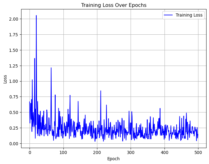
Because our training run logged the training loss as a history for each epoch, we can fetch the loss curve via the MLflow API and plot it ourselves.
Show the code
# Retrieve training loss history for the known run_idtrain_loss_history = client.get_metric_history(run.info.run_id, "train_loss")# Convert to a Pandas DataFrameloss_df = pd.DataFrame( [(m.step, m.value) for m in train_loss_history], columns=["epoch", "loss"])# Plot the training lossplt.figure(figsize=(8, 6))plt.plot(loss_df["epoch"], loss_df["loss"], label="Training Loss", color="blue")plt.xlabel("Epoch")plt.ylabel("Loss")plt.title("Training Loss Over Epochs")plt.legend()plt.grid()plt.show()
What else is there ?
We have only scratched the surface of what MLflow can do. It packs a lot of useful tools for managing your machine learning projects. It’s not just about tracking experiments — it also lets you deploy models, keep track of different versions, and even serve them. You can push your models to platforms like Azure ML, AWS SageMaker, or Databricks, and the model registry makes it easy to handle versioning, while the model server helps you put your models into production.
Here are some of other aspects we haven’t covered here which it can help with:
Automated Model Packaging: You can bundle your models along with all their dependencies using Conda or Docker, which really smooths out the deployment process.
Scalability: Whether you’re just tinkering with a prototype or launching a full-scale production system, MLflow integrates well with Kubernetes and cloud services.
Interoperability: It works with a bunch of popular ML frameworks like TensorFlow, Scikit-Learn, PyTorch, and XGBoost, so it fits into various workflows.
Hyperparameter Optimization: You can hook it up with tools like Optuna and Hyperopt to make tuning your models more systematic and efficient.
Model Registry: Keep track of model versions, artifacts, and metadata ensuring reproducibility and easier collaboration.